Model
The model chose for this reinforcement learning exercise was a Dueling Double Deep Q Network (D3QN). The D3QN is an extension of the Deep Q Network model, and seeks to improve the stability and efficiency of the learning process.
Lets break that down:
Q Learning and Network
Q values are state-action pairs. It represents the expected future rewards that an agent can get by taking that specific action in the given state. Consider the following example (adapted from TowardDataScience)
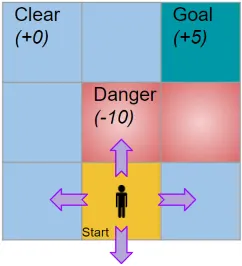
Hypothetical game environment
In this example, an agent starts in the start square of a 3x3 grid and hopes to reach the goal destination. Some of the squares provide no reward, while the danger and goal squares provide a reward of -10 and +5, respectively. Since the player can move into 9 squares, using four actions, a Q-table is made of 9 rows and 4 columns.
A Q-Learning algorithm would pick an action to use with the Epsilon-Greedy Policy. The Epsilon-Greedy policy is a exploration-exploitation strategy that balances picking new actions (Exploration) with choosing the best known action (Exploitation). After an action is picked, the agent obtains an observation from the environment. Then, the current Q-Value is updated using the observed reward. The target Q-value is the action with the maximum Q-value from the next state. This process of current action and target action finding is the basis of Q-Learning.
The update for a Q-Value for a chosen action is done with the equation \({\text{New}Q(s,a) = (1-\alpha)* Q(s,a) + \alpha * (r + \gamma * \text{max}_{a'}Q(s',a'))}\)
$Q(s,a)$ is the current estimate of the Q value for taking action $a$ in state $s$. $\alpha$ is the learning rate. $r$ is the reward gained from taking action $a$ in state $s$. $\gamma$ is the discount factor, which is used to determine the importance of future rewards. It makes the againt priortize immedeate rewards if $\gamma$ is closer to 0 and long-term rewards if $\gamma$ is closer to 1. $s’$ is the state of the environment after taking action $a$. Finally, $\text{max}_{a’}Q(s’,a’)$ is the maximum Q value over all possible actions $a’$ in the next state $s’$. This represents the potential maximum future rewards in the next state.
Q-Networks solve a problem that arises when using a table. For many real world scenarios, constructing a table of every possible action and state is near impossible. So, we use a Deep Q Network to model a Q-function that will map state and action pairs. Below is an example of the flow of a Deep Q Network each time step.
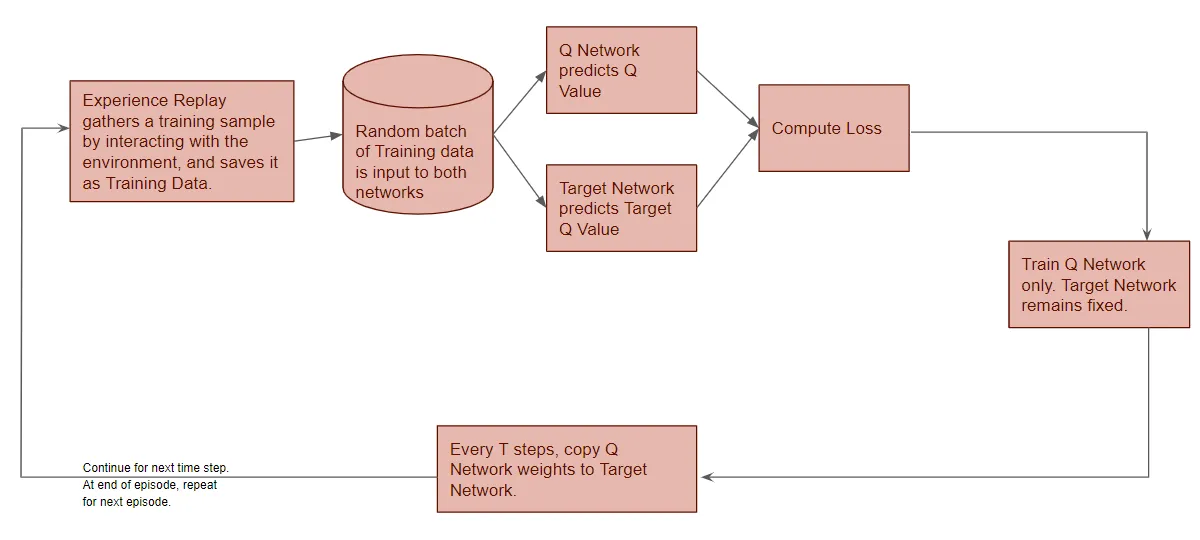
Diagram of how a Q Network runs
An important note is that the Experience Replay is needed to ensure the improvement of a network. Since neural networks generally perfrom best on a batch of random samples, the Experience Replay function provides that diversity n the training data.
Double Deep Q Network
Double Deep Q networks are an improvement to the overall architecture of Deep Q Networks. The main goal of this approach is to avoid an overestimation bias when estimating Q-Values. In a normal Deep Q Network, an overestimation bias can occur when the same set of data is used to both select and evaluate an action.
Double Deep Q Networks address that issue by using two separate sets of Q-values. The Double Deep Q network has two separate neural networks to establish action values. One network is used to select the action, and the other is used to evaluate that action. An updated equation for estimating Q-Value updates is shown below, \({\text{New}Q(s,a) = (1-\alpha)* Q(s,a) + \alpha * (r + \gamma * Q(s', \text{max}_{a'}Q(s',a')))}\)
where there are two different Q values chosen by two different networks.
Dueling Double Deep Q Network
A Dueling Double Deep Q Network (D3QN) is an extension of the Double Deep Q Network. A D3QN implements a dueling architecture, as noted by the name. A dueling architecture separates the estimation function and the value function. This is done by creating a Value Function, which represents the expected cumulative future rewards of being in a particular state, regardless of action taken. There is also an Advantage function, which represents the difference between the expected cumulative future rewards for taking an action and the value of the state. It captures the beneffit of taking a particular action in the given state. This is used in the D3QN to find the final Q value. Shown below is an example architecture of a D3QN.
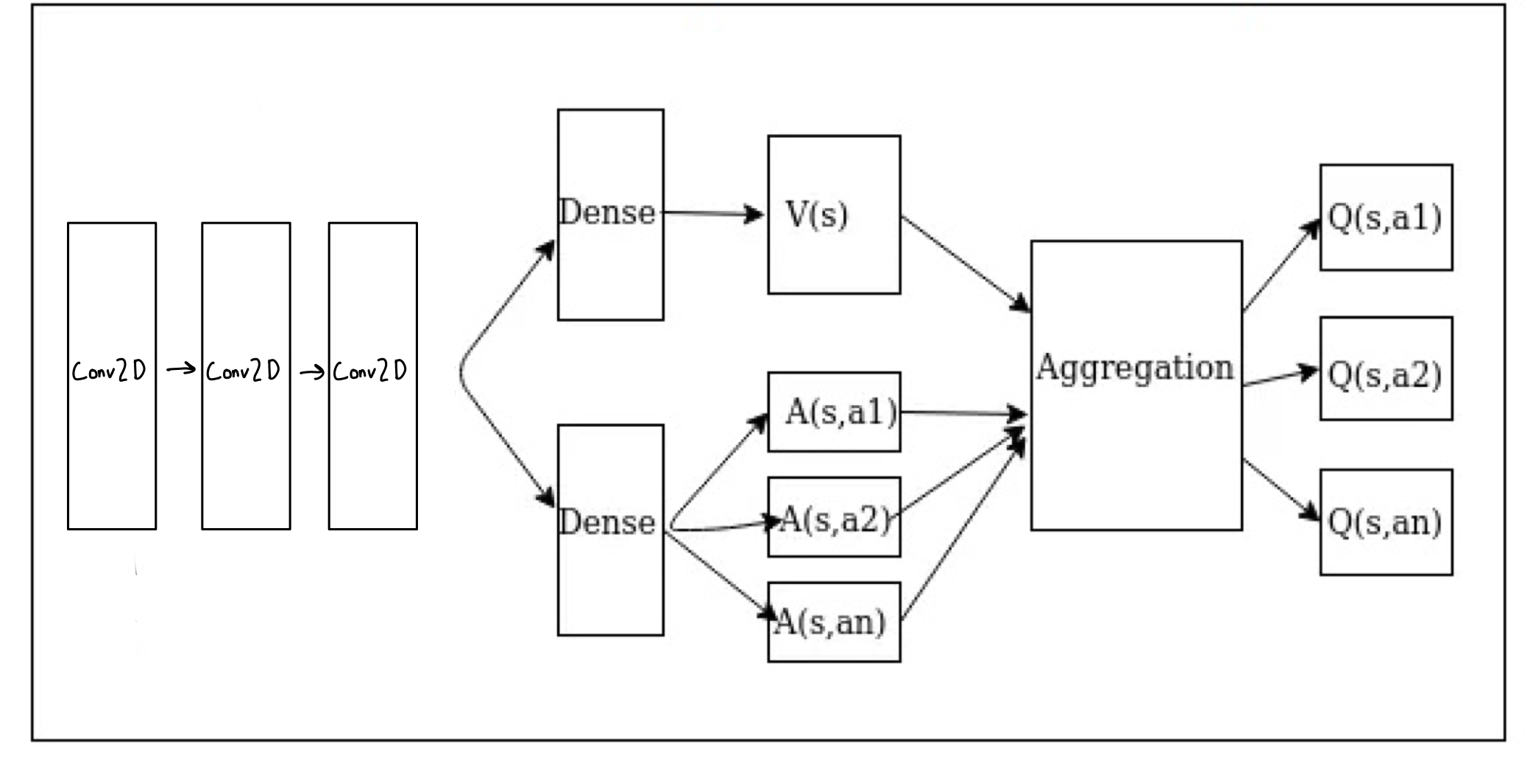
Architecture of a Dueling Double Deep Q Network
Method
For this project, I decided to try to implement the D3QN model using the gym_super_mario_bros package. This package provides an environment and emulator, as well as ROMs for several Super Mario Bros. games.
The first thing in the model is the ReplayBuffer class. This class is an important component of the D3QN as it stores a “memory” of the past experiences in the form of (state, action, reward, next_state, done). During training, the agent samples a batch of experiences and updates the paramaters based on those experiences. The buffer also has a constant size, which overwrites the oldest saved experiences with newer ones. I chose to use a deque system for my ReplayBuffer.
The next important implementation was my Agent class. The Agent class does many important things, chief among them building the D3QN model. The D3QN model consists of 3 Conv2D layers that are activated with ReLU. Then, there is a flatten layer, which prepares the data for the advantage and value streams. The advantage and value streams are both fully connected layers of 512 units. Next, a Python lambda combines the advantage and value streams. Finally, a Keras model is created, compiled, and returned. This function is shown below:
def _build_model(self):
        input_shape = self.observation_shape

        input_layer = Input(shape=input_shape)
        conv1 = Conv2D(32, (8, 8), strides=(4, 4), activation='relu')(input_layer)
        conv2 = Conv2D(64, (4, 4), strides=(2, 2), activation='relu')(conv1)
        conv3 = Conv2D(64, (3, 3), strides=(1, 1), activation='relu')(conv2)
        flattened = Flatten()(conv3)

        # Advantage streama
        fc_advantage = Dense(512, activation='elu', kernel_initializer='random_uniform')(flattened)
        advantage = Dense(self.action_size, activation='linear')(fc_advantage)

        # Value stream
        fc_value = Dense(512, activation='elu', kernel_initializer='random_uniform')(flattened)
        value = Dense(1, activation='linear')(fc_value)

        # Combine advantage and value to get final Q-values
        combined = Lambda(lambda x: x[1] + x[0] - K.mean(x[0], axis=1, keepdims=True), output_shape=(self.action_size,))([advantage, value])

        model = Model(inputs=input_layer, outputs=combined)
        model.compile(loss='mse', optimizer=Adam(lr=self.learning_rate))
        return model
Once the Agent class is made, the main loop is ready to be run. The main loop essentialy instatiates the model, loads in saved weights, if there are any, and begins the episodes. Additionally, there are options to record the training as well as render it so you can watch the model learn. Finally, at the conclusion, a graph is created showing reward history over the episodes.